How much more extraction risk do we find when we count near-verbatim cases?

Language models memorize some, but not all, of their training data. Intuitively, a piece of training data is memorized if the model assigns that specific text very high probability; this means that piece of training data is encoded in the model's weights in some form (Cooper and Grimmelmann, 2024; Carlini, 2025; Cooper et al., 2025). Arguably the most popular way to quantify memorization in LLMs is extraction: prompting the model so that it reproduces memorized training data in its outputs (Carlini et al., 2021). Studying memorization can tell us about model quality, since it may indicate overfitting rather than generalization. Memorization and extraction also have extensive implications for privacy and copyright.

Different ways of measuring extraction

The most common method is verbatim discoverable extraction (Lee et al., 2022; Carlini et al., 2023). For an open-weight base model, you take a piece of its training data, split it into a prefix and a target suffix, prompt the model with the prefix, generate a continuation with greedy decoding, and check whether that continuation exactly matches the target suffix. In practice, both are usually 50 tokens; the prefix prompt could be longer or shorter, but 50 tokens is the minimum length for outputs that the field tends to accept as valid evidence for extraction. Greedy decoding picks the single most likely (top-1) next token at every generation step, which makes it a cheap proxy for finding a high-probability continuation. It's also deterministic: for the same model, prefix, and continuation length, you get the same continuation every time.

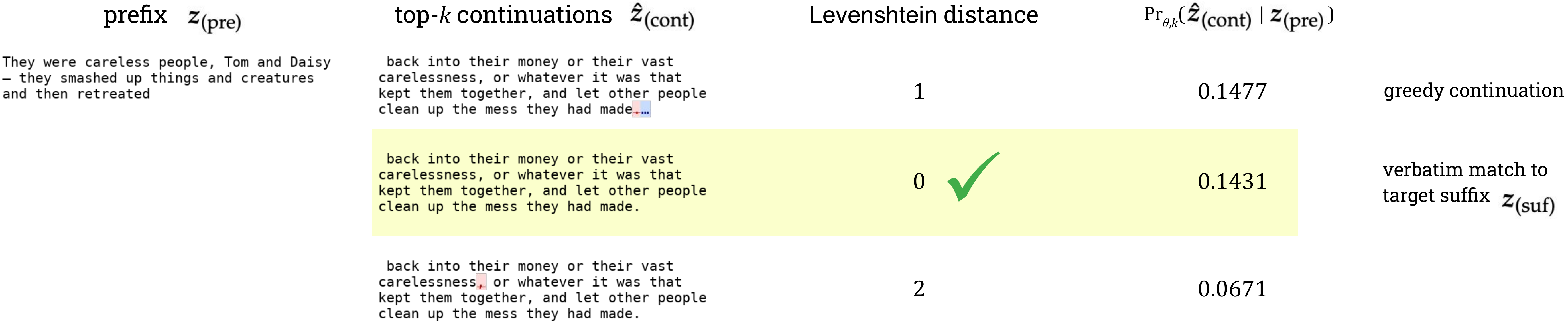
This setup naturally extends to near-verbatim extraction (Ippolito et al., 2023). Instead of requiring an exact match between the greedy continuation and the target suffix, you take that same continuation, measure its distance to the target suffix with a chosen distance metric (in either token or character space), and count it as extracted if it's within a small distance. Figure 1 shows an example, for Llama 1 13B and a training sequence from The Great Gatsby. The greedy continuation (top row) matches the target suffix except at the very end, where it has an ellipsis instead of a period.¹ This is just one punctuation difference from the verbatim target, so verbatim discoverable extraction wouldn't count it as extracted, but near-verbatim extraction would.

Recent work introduces a probabilistic relaxation of verbatim discoverable extraction (Hayes et al., 2025). Since memorization means a sequence has unusually high probability under the model, why not measure that probability directly? Concretely, we can easily compute the probability of generating the exact target suffix given the prefix under a chosen decoding scheme, and then count the sequence as extracted if that probability is at least some threshold, τ_min.² In Figure 1, the verbatim target suffix (highlighted) has probability 0.1431 under top-k decoding (k = 40), which ranks slightly below the probability of the greedy continuation.

This approach reveals significantly more memorization than its greedy, deterministic counterpart (Hayes et al., 2025; Cooper et al., 2025). It also conveys relative extraction risk across sequences, which greedy decoding can't. Two sequences might both count as extracted, but if one has probability 0.5 and the other 0.002, the first is far more likely to be generated: you'd expect to see it in about 2 samples, versus about 500 samples for the second. In contrast, greedy extraction would treat these two sequences the same way: it collapses extraction into the same binary, yes-or-no answer.

It's also significantly cheaper to compute at scale than greedy generation, in terms of wall-clock time. Instead of generating the continuation one token at a time, we can use teacher-forced inference: run a single forward pass over the entire 100-token sequence (the prefix and the target suffix), which gives the model's logits at every position at once. We can then cheaply post-process those logits to get the probability of each suffix token given everything before it, under whichever decoding policy we choose (for top-k, keep the k largest logits and renormalize). Multiplying those per-token probabilities gives the exact probability of the whole suffix.³

Teacher forcing is what makes probabilistic extraction efficient, but it doesn't naturally extend to the near-verbatim case. That's because it requires feeding the model a specific sequence: the full verbatim prefix and suffix. But for near-verbatim, there are many possible suffixes that could count as successful extraction. For instance, in Figure 1, all three continuations are near-verbatim matches, and there are many others. That makes the near-verbatim probability much trickier to compute.

And that's what this post is about. We've just walked through two overarching axes for measuring extraction: whether to use a deterministic (greedy) or probabilistic decoding scheme, and whether to require a verbatim match or accept a near-verbatim one.

In our new paper (Cooper et al., 2026a), we introduce an algorithm for the missing piece: efficiently estimating near-verbatim probabilistic extraction. The other three cells each give an exact answer: a greedy check is a definite yes or no, and teacher forcing gives the exact verbatim probability. In contrast, our near-verbatim probabilistic method returns a deterministic lower bound, for about the cost of 20 samples. Settling for a lower bound is what keeps our approach tractable, because, as we'll see next, computing the near-verbatim probability exactly is far too expensive.

The obvious ways to compute near-verbatim probabilities are expensive

To compute a near-verbatim extraction probability, we first need to pin down which continuations count as "near-verbatim." Given a target suffix, a distance function, and a small maximum distance ε, the near-verbatim ball around the target suffix is the set of every continuation within ε of it. The near-verbatim probability is the total probability of everything in the near-verbatim ball: the sum of the probabilities of all of those continuations. As with verbatim probabilistic extraction, a sequence counts as extracted if this probability is at least τ_min.

To make this concrete, we use an illustrative example, which we also use in the walk-throughs below: a prefix from The Great Gatsby (which is in the training data) and its 8-word target suffix.

prefixsmashed up things and creatures and then retreated

target suffixback into their money or their vast carelessness

Here, for simplicity, one word is one token, and the numbers are illustrative; they aren't from a real model.

Which continuations land in the near-verbatim ball depends on the distance function. Hamming distance compares two equal-length sequences position by position, and counts the positions where they differ. Levenshtein distance counts the fewest edits (substitutions, insertions, or deletions) needed to change one sequence into the other. Levenshtein is more forgiving of shifts: a continuation that skips the first word of the target suffix but otherwise matches is off by one at every position, so its Hamming distance is large, but its Levenshtein distance is just 2: insert the missing word at the start, and delete the extra word at the end (Figure 2).

For this example target suffix, the Levenshtein ball with ε = 2 contains every 8-word continuation within 2 edits of it. Figure 3 visualizes the Levenshtein ball, showing a few of the continuations that are 1 or 2 edits away, along with their probabilities given the prefix. (Remember that these numbers are illustrative; this example doesn't use a real model.) Some are plausible, like back to their money or their vast carelessness (probability 0.081); others, like back github their money or their vast carelessness, have probability 0. The exact near-verbatim probability is the sum of the probabilities of all the sequences in the whole near-verbatim ball.

Exact computation is intractable

In principle, we could compute the near-verbatim probability exactly: list every continuation in the near-verbatim ball, teacher-force each one (appended to the prefix) to get its exact conditional probability, and add them all up. But in practice, the near-verbatim ball is far too large to do this. For our small 8-word example, with a 32,000-word vocabulary, the Hamming ball within 2 edits contains on the order of 10¹⁰ continuations. For a 50-token suffix with a 32,000-token vocabulary (Llama 2's, for example), it's on the order of 10¹² sequences. (In general, the Levenshtein ball for the same number of edits is even larger.)

Teacher-forcing every one of these sequences just isn't possible, and it also shouldn't be necessary. Most of the near-verbatim ball has little or no probability. As in Figure 3, a continuation like back github their money or their vast carelessness is technically within 2 edits of the target suffix, but under top-k decoding it can't even be generated at all. Ideally, we'd spend computation only on the small part of the near-verbatim ball that actually carries probability, since what we care about for extraction is whether the near-verbatim probability is unusually high.

Estimating via Monte Carlo sampling is infeasible

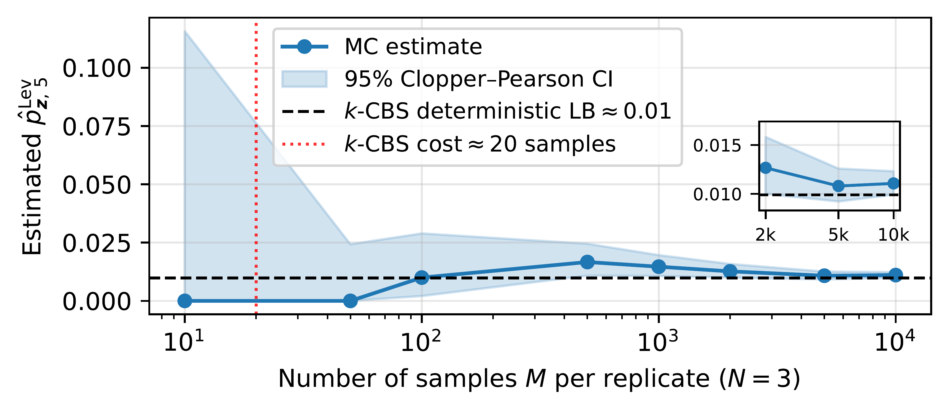
Rather than computing the near-verbatim probability exactly, we could estimate it by sampling. Generate many continuations from the prefix under the decoding policy, check each one's distance to the target suffix, and estimate the near-verbatim probability as the fraction that land within ε. This Monte Carlo (MC) estimate is unbiased, and with enough samples, it converges to the true probability; continuations with high probability should show up often. The catch is what counts as "high." For a 50-token suffix, a near-verbatim probability of 0.01 is enormous for an LLM, and very likely a sign of extraction, but it's small in absolute terms. You'd need about 100 samples on average just to land in the near-verbatim ball once, and many more to estimate the probability reliably.

Figure 4 shows this for one 50-token suffix from The Great Gatsby with Llama 2 7B, using Levenshtein distance with ε = 5; there, MC's estimate for the near-verbatim probability eventually settles near 0.01. With 10 or 50 samples, MC never lands in the near-verbatim ball, so it estimates 0. With 100, it starts to find some, but the confidence interval is still wide, and it takes thousands of samples for the estimate to settle near 0.01. In contrast, our approach (k-CBS) gets a deterministic lower bound that's close to the MC estimate after 10,000 samples, for the cost of about 20 samples.

Top-k-constrained beam search (k-CBS), step by step

The intuition behind our approach is simple. Beam search is a standard decoding algorithm that tends to find continuations with high probability under the model. Memorized suffixes have unusually high probability. So when a sequence is memorized, beam search should find continuations in its near-verbatim ball. Like greedy decoding, beam search generates one token at a time, but instead of committing to the single most likely token, it keeps the B most probable partial continuations so far: the beam, of beam width B. At each step, it extends each of them by every possible next token, and keeps only the B highest-scoring results. Since a continuation's probability is a product over steps, only continuations whose probability stays among the highest at every step survive. So beam search concentrates its effort on a thin, high-probability slice of the possible continuations, without exploring all of them.

Our approach, decoding-constrained beam search (CBS), modifies beam search to work under a given decoding policy, so it returns continuations along with their exact probabilities under that policy. CBS can work with other decoding policies; we focus on top-k decoding with k = 40 and temperature 1, since this is the main setting studied in prior work on probabilistic extraction (Hayes et al., 2025; Cooper et al., 2025). This version, top-k-constrained beam search (k-CBS), makes three changes to beam search:

1. It extends each partial continuation only by its k most likely next tokens, since under top-k decoding no other token can be generated.
2. It scores continuations by their probability under top-k decoding, renormalizing each step's top k probabilities to sum to 1.
3. At the last step, it keeps all B · k final candidates instead of cutting back to B. The last step of beam search has already produced those candidates, and they're all valid continuations under the decoding policy, so it costs no extra model calls to retain them.

The animation below steps through k-CBS on the illustrative example from Figure 3: the same prefix, target suffix, and made-up model. To keep it small, it uses k = 5, a beam of B = 3, and ε = 2 on 8-word suffixes. (The experiments in the paper use k = 40, B = 20, and ε = 5 on 50-token suffixes.) The animation also prunes partial continuations during the search, once they can no longer end within 2 edits (Levenshtein distance) of the target suffix; we describe this further below. Step through it with the buttons below it, or with the left and right arrow keys; hitting the spacebar plays and pauses.

At the end, k-CBS adds up the probabilities of the returned continuations that are within ε of the target suffix. Every probability in that sum is exact, and every continuation in it is in the near-verbatim ball, so the sum is a deterministic lower bound on the near-verbatim probability. It's only a lower bound because, along the way, the search can cut continuations outside the top-B that could've ended up in the near-verbatim ball if they were expanded to the end; their probability never makes it into the sum. But for memorized sequences, we observe that the bound tends to be very useful in practice: a continuation with enough probability to indicate memorization has to pick one of the top-ranked tokens at almost every step, which is exactly the part of the space that k-CBS explores. In Figure 4, k-CBS recovers 89.4% of the probability that MC finds after 10,000 samples. And with B = 20, as in our experiments, it costs about as much as 20 MC samples.

k-CBS can also prune as it goes, which is what the animation does. If a partial continuation already needs more than ε edits to match the target suffix, no matter which tokens come next, there's no point keeping it in the beam: it can never end up in the near-verbatim ball, and it takes a slot from a continuation that perhaps still could. Pruning is optional, and it only works with distances with certain properties.⁴ (The pruned versions only return candidates within ε, so there's no need to filter before summing up their probabilities.) For the Hamming distance, it's simple: keep a running count of the positions that don't match the target suffix. That count can only go up, so once it's more than ε, the continuation can't be in the near-verbatim ball. Levenshtein distance is trickier, since a later insertion or deletion can line up words that looked mismatched (Figure 2). For Levenshtein, k-CBS uses a dynamic program, which we walk through next.

Pruning with Levenshtein

For Levenshtein distance, k-CBS keeps track of every way the continuation so far could line up with the start of the target suffix, using a classic dynamic program (Wagner and Fischer, 1974). The dynamic program fills in a table, with one row per generated token and one column per token of the target suffix: each cell holds the fewest edits needed to change the continuation so far into the target suffix up to that column. (For two sequences of T tokens, we don't need the full (T + 1) × (T + 1) table: it's enough to keep the diagonal band of at most 2ε + 1 cells per row; see Ukkonen, 1985 and Navarro, 2001.)

The smallest number in the newest row is what the k-CBS animation calls min. edits: the fewest edits the finished continuation could need to match the target suffix, no matter which tokens come next. As more tokens are generated, min. edits can stay the same or go up (but not down).⁵ So once it's more than ε, the continuation can be pruned.

To understand the state the dynamic program maintains to determine min. edits, step through the animation with the buttons below it, or with the left and right arrow keys; hitting the spacebar plays and pauses. You can pick from three continuations: one that matches verbatim, the one-word shift from Figure 2, and one that gets pruned because its min. edits exceed ε = 2.

Near-verbatim reveals more extracted sequences and increased risk

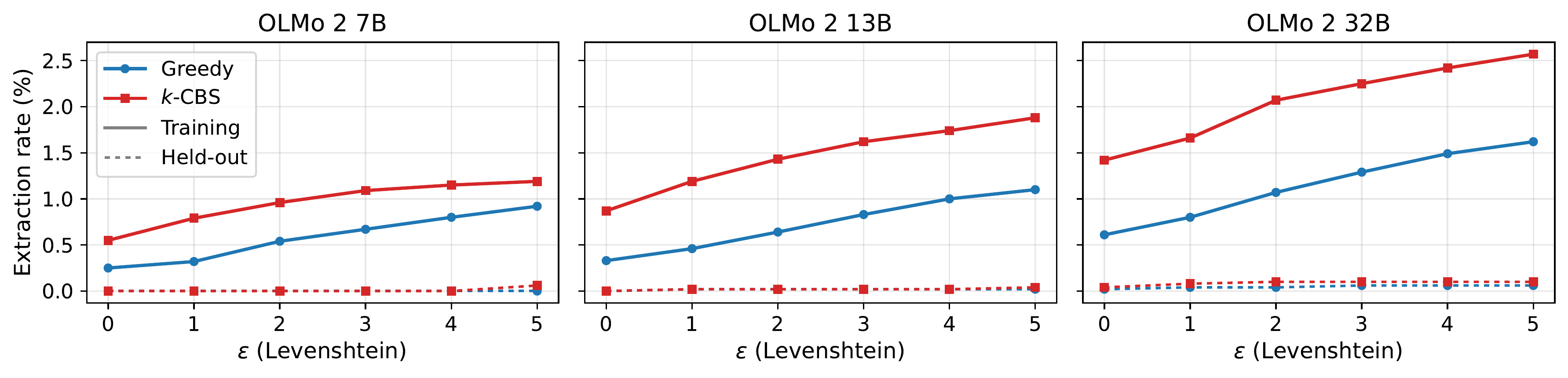
Accounting for near-verbatim matches reveals substantially more extraction, in two ways: more sequences count as extracted, and individual sequences may carry much more extraction risk. Figure 5 shows the first, for OLMo 2 on Wikipedia: k-CBS finds more extraction than greedy at every ε and model size.

The gap grows with model size (that is, the difference between greedy and probabilistic extraction rates gets wider as models get larger). For OLMo 2 32B at ε = 5, 2.57% of sequences are extractable, compared with 1.42% for verbatim probabilistic extraction and 0.61% for greedy verbatim extraction.⁶ As a negative control, we also run the same experiments on non-training data (labeled "Held-out" in the figure): Wikipedia entries written after the models' training cutoff. By definition, the models can't have memorized non-training data, so for our extraction procedure to be valid, the rates need to (and do) stay near zero.⁷

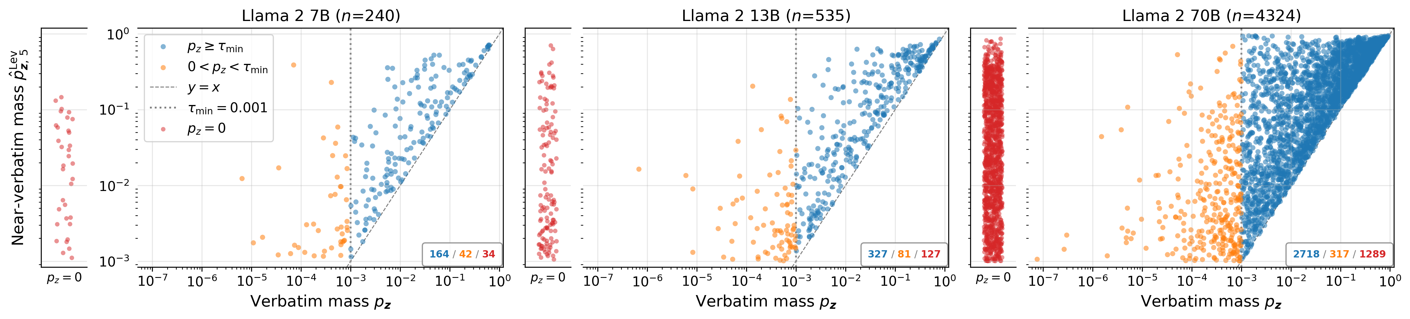
Figure 6 shows the second, for Llama 2 on The Great Gatsby. Each point is one sequence, with its near-verbatim probability (Levenshtein, ε = 5) plotted against its verbatim probability. The orange and red points are sequences that verbatim probabilistic extraction misses, because their verbatim probability is below τ_min (orange) or exactly 0 (red), but that are extractable once near-verbatim continuations are accounted for. At 70B, 1,606 sequences are "unlocked" this way, and 1,289 of them have zero verbatim probability. And these unlocked sequences aren't borderline cases: on average, their near-verbatim probability is 0.086, which is 86 times τ_min. Often the only difference from the target is something tiny, like spacing around punctuation. The blue points are already verbatim-extractable; those above the dashed line carry more risk once we account for near-verbatim continuations.

In the paper, we also run experiments on other model families and kinds of text, including Pythia on emails and Llama 2 on other books. Accounting for near-verbatim extraction, we observe different patterns in how extraction risk changes with model size, depending on the type of text being analyzed. These two figures are just a preview; see the paper for those results and more.

How to cite our work

@inproceedings{cooper2026nv,
  title     = {Estimating near-verbatim extraction risk in language models with
               decoding-constrained beam search},
  author    = {Cooper, A. Feder and Lemley, Mark and De Sa, Christopher and
               Duesterwald, Lea and Casasola, Allison and Hayes, Jamie and
               Lee, Katherine and Ho, Daniel E. and Liang, Percy},
  booktitle = {Third Conference on Language Modeling},
  year      = {2026},
  url       = {https://openreview.net/forum?id=05XN0gq1Z7}
}

This work was supported by a Stanford University Human-Centered Artificial Intelligence (HAI) seed grant, "Assessing Copyright Risks of Training Data 'Memorization' and 'Extraction' for Open-Weight Language Models."